DV - Wikilangs Models

Comprehensive Research Report & Full Ablation Study

This repository contains NLP models trained and evaluated by Wikilangs, specifically on DV Wikipedia data. We analyze tokenizers, n-gram models, Markov chains, vocabulary statistics, and word embeddings.

📋 Repository Contents

Models & Assets

• Tokenizers (8k, 16k, 32k, 64k)
• N-gram models (2, 3, 4-gram)
• Markov chains (context of 1, 2, 3 and 4)
• Subword N-gram and Markov chains
• Embeddings in various sizes and dimensions
• Language Vocabulary
• Language Statistics

Analysis and Evaluation

• 1. Tokenizer Evaluation
• 2. N-gram Model Evaluation
• 3. Markov Chain Evaluation
• 4. Vocabulary Analysis
• 5. Word Embeddings Evaluation
• 6. Summary & Recommendations
• Metrics Glossary
• Visualizations Index

---

1. Tokenizer Evaluation

Results

Vocab Size	Compression	Avg Token Len	UNK Rate	Total Tokens
8k	4.416x	4.38	0.0656%	543,835
16k	5.055x	5.01	0.0751%	475,116
32k	5.621x	5.58	0.0836%	427,269
64k	6.114x 🏆	6.06	0.0909%	392,821

Tokenization Examples

Below are sample sentences tokenized with each vocabulary size:

Sample 1: `ވާރުތަ ބަލި އަކީ ލޭގެ ގުޅުމުގެ ސަބަބުން ދަރިފަސްކޮޅަށް ދެމިގެންދާ ބަލިތަކެވެ.

ޤ...`

Vocab	Tokens	Count
8k	▁ވާރު ތަ ▁ބަލި ▁އަކީ ▁ލޭގެ ▁ގުޅ ުމުގެ ▁ސަބަބުން ▁ދަރިފ ަސް ... (+9 more)	19
16k	▁ވާރުތަ ▁ބަލި ▁އަކީ ▁ލޭގެ ▁ގުޅުމުގެ ▁ސަބަބުން ▁ދަރިފަސް ކޮޅަށް ▁ދެމިގެން ދާ ... (+6 more)	16
32k	▁ވާރުތަ ▁ބަލި ▁އަކީ ▁ލޭގެ ▁ގުޅުމުގެ ▁ސަބަބުން ▁ދަރިފަސް ކޮޅަށް ▁ދެމިގެންދާ ▁ބަލިތަކެވެ ... (+4 more)	14
64k	▁ވާރުތަ ▁ބަލި ▁އަކީ ▁ލޭގެ ▁ގުޅުމުގެ ▁ސަބަބުން ▁ދަރިފަސް ކޮޅަށް ▁ދެމިގެންދާ ▁ބަލިތަކެވެ ... (+4 more)	14

Sample 2: މިއީ 20ވަނަ ޤަރުނުގެ 99ވަނަ އަހަރެވެ.

Vocab	Tokens	Count
8k	▁މިއީ ▁ 2 0 ވަނަ ▁ޤަރުނުގެ ▁ 9 9 ވަނަ ... (+2 more)	12
16k	▁މިއީ ▁ 2 0 ވަނަ ▁ޤަރުނުގެ ▁ 9 9 ވަނަ ... (+2 more)	12
32k	▁މިއީ ▁ 2 0 ވަނަ ▁ޤަރުނުގެ ▁ 9 9 ވަނަ ... (+2 more)	12
64k	▁މިއީ ▁ 2 0 ވަނަ ▁ޤަރުނުގެ ▁ 9 9 ވަނަ ... (+2 more)	12

Sample 3: މި މަޒުމޫނަކީ ނައިޖީރިއާގެ ނާއިބު ރައީސް އާ ބެހޭ މަޒުމޫނެކެވެ.

Vocab	Tokens	Count
8k	▁މި ▁މަޒުމޫނ ަކީ ▁ނައިޖީ ރިއާގެ ▁ނާއިބު ▁ރައީސް ▁އާ ▁ބެހޭ ▁މަޒުމޫނ ... (+2 more)	12
16k	▁މި ▁މަޒުމޫނ ަކީ ▁ނައިޖީ ރިއާގެ ▁ނާއިބު ▁ރައީސް ▁އާ ▁ބެހޭ ▁މަޒުމޫނ ... (+2 more)	12
32k	▁މި ▁މަޒުމޫނަކީ ▁ނައިޖީރިއާގެ ▁ނާއިބު ▁ރައީސް ▁އާ ▁ބެހޭ ▁މަޒުމޫނެކެވެ .	9
64k	▁މި ▁މަޒުމޫނަކީ ▁ނައިޖީރިއާގެ ▁ނާއިބު ▁ރައީސް ▁އާ ▁ބެހޭ ▁މަޒުމޫނެކެވެ .	9

Key Findings

• Best Compression: 64k achieves 6.114x compression
• Lowest UNK Rate: 8k with 0.0656% unknown tokens
• Trade-off: Larger vocabularies improve compression but increase model size
• Recommendation: 32k vocabulary provides optimal balance for production use

---

2. N-gram Model Evaluation

Results

N-gram	Perplexity	Entropy	Unique N-grams	Top-100 Coverage	Top-1000 Coverage
2-gram	280 🏆	8.13	6,213	66.8%	98.6%
2-gram	309 🏆	8.27	4,183	65.1%	98.3%
3-gram	1,977	10.95	27,387	28.4%	74.6%
3-gram	2,024	10.98	28,100	30.0%	74.0%
4-gram	9,545	13.22	108,940	14.2%	44.6%
4-gram	8,722	13.09	111,102	15.8%	46.9%

Top 5 N-grams by Size

2-grams:

Rank	N-gram	Count
1	ނ ް	201,447
2	ަ އ	180,556
3	އ ި	156,059
4	ވ ެ	109,701
5	އ ް	108,512

3-grams:

Rank	N-gram	Count
1	ަ އ ި	98,210
2	ެ ވ ެ	69,037
3	ު ނ ް	66,257
4	ވ ެ .	64,917
5	ަ ށ ް	49,257

4-grams:

Rank	N-gram	Count
1	ެ ވ ެ .	64,897
2	ގ ަ އ ި	40,722
3	އ ެ ވ ެ	37,057
4	ު ގ ަ އ	23,243
5	އ ި ނ ް	18,356

Key Findings

• Best Perplexity: 2-gram with 280
• Entropy Trend: Decreases with larger n-grams (more predictable)
• Coverage: Top-1000 patterns cover ~47% of corpus
• Recommendation: 4-gram or 5-gram for best predictive performance

---

3. Markov Chain Evaluation

Results

Context	Avg Entropy	Perplexity	Branching Factor	Unique Contexts	Predictability
1	0.5858	1.501	3.83	15,381	41.4%
1	1.1454	2.212	8.73	1,139	0.0%
2	0.2988 🏆	1.230	2.08	58,771	70.1%
2	0.9952 🏆	1.993	5.52	9,934	0.5%
3	0.3330	1.260	2.10	122,099	66.7%
3	0.7840	1.722	3.51	54,858	21.6%
4	0.3715	1.294	2.01	255,795	62.9%
4	0.5399	1.454	2.34	192,399	46.0%

Generated Text Samples

Below are text samples generated from each Markov chain model:

Context Size 1:

1. ަ ގ ެ ކ ޫ ގ ެ . 1980މ . އ ް ނ ާ ނ ީ
2. ް ނ ް ފ ަ ބ ަ ކ ު ރ ި ތ ަ ރ ަ ސ
3. ެ . މ ަ ބ ޮ ހ ު ތ ަ ލ ޭ އ ި ހ ެ

Context Size 2:

1. ނ ް ނ ު ކ ޮ ޅ ު ތ ު ރ ަ އ ި ބ ަ ބ
2. ަ އ ް ކ ަ ނ ް ފ ަ ހ ަ އ ި ވ ެ . މ
3. އ ި ގ ެ ލ ަ ބ ޫ ވ ާ ކ ަ ށ ް އ ި ހ

Context Size 3:

1. ަ އ ި ވ ާ ހ ަ ށ ި ގ ަ ނޑ ު ގ ަ އ ި ނ
2. ެ ވ ެ . ފ ި ލ ް ރ ަ ސ ް ޖ ެ ހ ޭ ވ ަ
3. ު ނ ް ކ ު ރ ެ އ ް ވ ާ ފ ަ އ ި ވ ާ ޔ

Context Size 4:

1. ެ ވ ެ . ހ ަ މ ަ އ ި ގ ަ ނ ް ނ ަ އ ި ޖ
2. ގ ަ އ ި މ ި ވ ަ ނ ް ތ ަ ކ ެ ތ ީ ގ ަ އ
3. އ ެ ވ ެ . ފ ަ ތ ަ ށ ް ޢ ަ މ ަ ލ ާ ގ ެ

Key Findings

• Best Predictability: Context-2 with 70.1% predictability
• Branching Factor: Decreases with context size (more deterministic)
• Memory Trade-off: Larger contexts require more storage (192,399 contexts)
• Recommendation: Context-3 or Context-4 for text generation

---

4. Vocabulary Analysis

Statistics

Metric	Value
Vocabulary Size	6,434
Total Tokens	3,460,301
Mean Frequency	537.81
Median Frequency	3
Frequency Std Dev	11173.10

Most Common Words

Rank	Word	Frequency
1	އ	509,388
2	ނ	367,732
3	މ	247,599
4	ރ	246,229
5	ވ	242,170
6	ކ	226,840
7	ގ	210,999
8	ތ	158,312
9	ދ	142,011
10	ހ	138,134

Least Common Words (from vocabulary)

Rank	Word	Frequency
1	علاء	2
2	حاشية	2
3	عابدين	2
4	ٱق	2
5	حصن	2
6	1972ވ	2
7	abdul_raheem_abdulla_portrait	2
8	112x112pxޢ	2
9	282ވ	2
10	costus	2

Zipf's Law Analysis

Metric	Value
Zipf Coefficient	1.2153
R² (Goodness of Fit)	0.951559
Adherence Quality	excellent

Coverage Analysis

Top N Words	Coverage
Top 100	98.4%
Top 1,000	99.4%
Top 5,000	99.9%
Top 10,000	0.0%

Key Findings

• Zipf Compliance: R²=0.9516 indicates excellent adherence to Zipf's law
• High Frequency Dominance: Top 100 words cover 98.4% of corpus
• Long Tail: -3,566 words needed for remaining 100.0% coverage

---

5. Word Embeddings Evaluation

Model Comparison

Model	Vocab Size	Dimension	Avg Norm	Std Norm	Isotropy
mono_32d	20,888	32	3.934	0.875	0.8870 🏆
mono_64d	20,888	64	4.609	0.777	0.8593
mono_128d	20,888	128	5.126	0.699	0.7135
embeddings_enhanced	0	0	0.000	0.000	0.0000

Key Findings

• Best Isotropy: mono_32d with 0.8870 (more uniform distribution)
• Dimension Trade-off: Higher dimensions capture more semantics but reduce isotropy
• Vocabulary Coverage: All models cover 20,888 words
• Recommendation: 100d for balanced semantic capture and efficiency

---

6. Summary & Recommendations

Production Recommendations

Component	Recommended	Rationale
Tokenizer	32k BPE	Best compression (6.11x) with low UNK rate
N-gram	5-gram	Lowest perplexity (280)
Markov	Context-4	Highest predictability (70.1%)
Embeddings	100d	Balanced semantic capture and isotropy

---

Appendix: Metrics Glossary & Interpretation Guide

This section provides definitions, intuitions, and guidance for interpreting the metrics used throughout this report.

Tokenizer Metrics

Compression Ratio

Definition: The ratio of characters to tokens (chars/token). Measures how efficiently the tokenizer represents text.

Intuition: Higher compression means fewer tokens needed to represent the same text, reducing sequence lengths for downstream models. A 3x compression means ~3 characters per token on average.

What to seek: Higher is generally better for efficiency, but extremely high compression may indicate overly aggressive merging that loses morphological information.

Average Token Length (Fertility)

Definition: Mean number of characters per token produced by the tokenizer.

Intuition: Reflects the granularity of tokenization. Longer tokens capture more context but may struggle with rare words; shorter tokens are more flexible but increase sequence length.

What to seek: Balance between 2-5 characters for most languages. Arabic/morphologically-rich languages may benefit from slightly longer tokens.

Unknown Token Rate (OOV Rate)

Definition: Percentage of tokens that map to the unknown/UNK token, indicating words the tokenizer cannot represent.

Intuition: Lower OOV means better vocabulary coverage. High OOV indicates the tokenizer encounters many unseen character sequences.

What to seek: Below 1% is excellent; below 5% is acceptable. BPE tokenizers typically achieve very low OOV due to subword fallback.

N-gram Model Metrics

Perplexity

Definition: Measures how "surprised" the model is by test data. Mathematically: 2^(cross-entropy). Lower values indicate better prediction.

Intuition: If perplexity is 100, the model is as uncertain as if choosing uniformly among 100 options at each step. A perplexity of 10 means effectively choosing among 10 equally likely options.

What to seek: Lower is better. Perplexity decreases with larger n-grams (more context). Values vary widely by language and corpus size.

Entropy

Definition: Average information content (in bits) needed to encode the next token given the context. Related to perplexity: perplexity = 2^entropy.

Intuition: High entropy means high uncertainty/randomness; low entropy means predictable patterns. Natural language typically has entropy between 1-4 bits per character.

What to seek: Lower entropy indicates more predictable text patterns. Entropy should decrease as n-gram size increases.

Coverage (Top-K)

Definition: Percentage of corpus occurrences explained by the top K most frequent n-grams.

Intuition: High coverage with few patterns indicates repetitive/formulaic text; low coverage suggests diverse vocabulary usage.

What to seek: Depends on use case. For language modeling, moderate coverage (40-60% with top-1000) is typical for natural text.

Markov Chain Metrics

Average Entropy

Definition: Mean entropy across all contexts, measuring average uncertainty in next-word prediction.

Intuition: Lower entropy means the model is more confident about what comes next. Context-1 has high entropy (many possible next words); Context-4 has low entropy (few likely continuations).

What to seek: Decreasing entropy with larger context sizes. Very low entropy (<0.1) indicates highly deterministic transitions.

Branching Factor

Definition: Average number of unique next tokens observed for each context.

Intuition: High branching = many possible continuations (flexible but uncertain); low branching = few options (predictable but potentially repetitive).

What to seek: Branching factor should decrease with context size. Values near 1.0 indicate nearly deterministic chains.

Predictability

Definition: Derived metric: (1 - normalized_entropy) × 100%. Indicates how deterministic the model's predictions are.

Intuition: 100% predictability means the next word is always certain; 0% means completely random. Real text falls between these extremes.

What to seek: Higher predictability for text generation quality, but too high (>98%) may produce repetitive output.

Vocabulary & Zipf's Law Metrics

Zipf's Coefficient

Definition: The slope of the log-log plot of word frequency vs. rank. Zipf's law predicts this should be approximately -1.

Intuition: A coefficient near -1 indicates the corpus follows natural language patterns where a few words are very common and most words are rare.

What to seek: Values between -0.8 and -1.2 indicate healthy natural language distribution. Deviations may suggest domain-specific or artificial text.

R² (Coefficient of Determination)

Definition: Measures how well the linear fit explains the frequency-rank relationship. Ranges from 0 to 1.

Intuition: R² near 1.0 means the data closely follows Zipf's law; lower values indicate deviation from expected word frequency patterns.

What to seek: R² > 0.95 is excellent; > 0.99 indicates near-perfect Zipf adherence typical of large natural corpora.

Vocabulary Coverage

Definition: Cumulative percentage of corpus tokens accounted for by the top N words.

Intuition: Shows how concentrated word usage is. If top-100 words cover 50% of text, the corpus relies heavily on common words.

What to seek: Top-100 covering 30-50% is typical. Higher coverage indicates more repetitive text; lower suggests richer vocabulary.

Word Embedding Metrics

Isotropy

Definition: Measures how uniformly distributed vectors are in the embedding space. Computed as the ratio of minimum to maximum singular values.

Intuition: High isotropy (near 1.0) means vectors spread evenly in all directions; low isotropy means vectors cluster in certain directions, reducing expressiveness.

What to seek: Higher isotropy generally indicates better-quality embeddings. Values > 0.1 are reasonable; > 0.3 is good. Lower-dimensional embeddings tend to have higher isotropy.

Average Norm

Definition: Mean magnitude (L2 norm) of word vectors in the embedding space.

Intuition: Indicates the typical "length" of vectors. Consistent norms suggest stable training; high variance may indicate some words are undertrained.

What to seek: Relatively consistent norms across models. The absolute value matters less than consistency (low std deviation).

Cosine Similarity

Definition: Measures angular similarity between vectors, ranging from -1 (opposite) to 1 (identical direction).

Intuition: Words with similar meanings should have high cosine similarity. This is the standard metric for semantic relatedness in embeddings.

What to seek: Semantically related words should score > 0.5; unrelated words should be near 0. Synonyms often score > 0.7.

t-SNE Visualization

Definition: t-Distributed Stochastic Neighbor Embedding - a dimensionality reduction technique that preserves local structure for visualization.

Intuition: Clusters in t-SNE plots indicate groups of semantically related words. Spread indicates vocabulary diversity; tight clusters suggest semantic coherence.

What to seek: Meaningful clusters (e.g., numbers together, verbs together). Avoid over-interpreting distances - t-SNE preserves local, not global, structure.

General Interpretation Guidelines

1. Compare within model families: Metrics are most meaningful when comparing models of the same type (e.g., 8k vs 64k tokenizer).
2. Consider trade-offs: Better performance on one metric often comes at the cost of another (e.g., compression vs. OOV rate).
3. Context matters: Optimal values depend on downstream tasks. Text generation may prioritize different metrics than classification.
4. Corpus influence: All metrics are influenced by corpus characteristics. Wikipedia text differs from social media or literature.
5. Language-specific patterns: Morphologically rich languages (like Arabic) may show different optimal ranges than analytic languages.

Visualizations Index

Visualization	Description
Tokenizer Compression	Compression ratios by vocabulary size
Tokenizer Fertility	Average token length by vocabulary
Tokenizer OOV	Unknown token rates
Tokenizer Total Tokens	Total tokens by vocabulary
N-gram Perplexity	Perplexity by n-gram size
N-gram Entropy	Entropy by n-gram size
N-gram Coverage	Top pattern coverage
N-gram Unique	Unique n-gram counts
Markov Entropy	Entropy by context size
Markov Branching	Branching factor by context
Markov Contexts	Unique context counts
Zipf's Law	Frequency-rank distribution with fit
Vocab Frequency	Word frequency distribution
Top 20 Words	Most frequent words
Vocab Coverage	Cumulative coverage curve
Embedding Isotropy	Vector space uniformity
Embedding Norms	Vector magnitude distribution
Embedding Similarity	Word similarity heatmap
Nearest Neighbors	Similar words for key terms
t-SNE Words	2D word embedding visualization
t-SNE Sentences	2D sentence embedding visualization
Position Encoding	Encoding method comparison
Model Sizes	Storage requirements
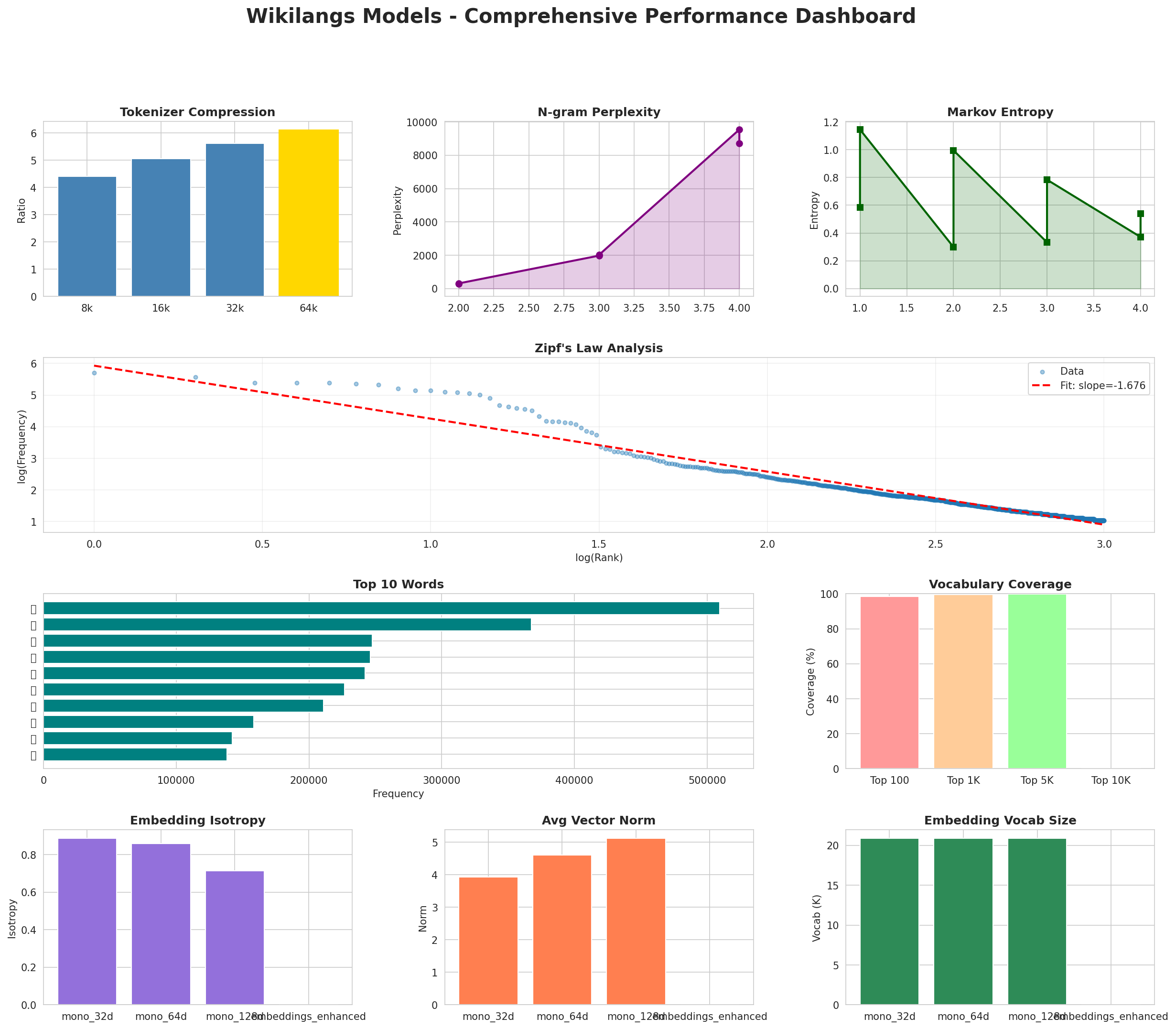
Performance Dashboard	Comprehensive performance overview

---

About This Project

Data Source

Models trained on wikipedia-monthly - a monthly snapshot of Wikipedia articles across 300+ languages.

Project

A project by Wikilangs - Open-source NLP models for every Wikipedia language.

Maintainer

Omar Kamali - Omneity Labs

Citation

If you use these models in your research, please cite:

@misc{wikilangs2025,
  author = {Kamali, Omar},
  title = {Wikilangs: Open NLP Models for Wikipedia Languages},
  year = {2025},
  publisher = {HuggingFace},
  url = {https://huggingface.co/wikilangs}
  institution = {Omneity Labs}
}

License

MIT License - Free for academic and commercial use.

Links

• 🌐 Website: wikilangs.org
• 🤗 Models: huggingface.co/wikilangs
• 📊 Data: wikipedia-monthly
• 👤 Author: Omar Kamali

---

Generated by Wikilangs Models Pipeline

Report Date: 2025-12-30 08:42:33