20x Faster TRL Fine-tuning with RapidFire AI


Authored by: RapidFire AI Team
This tutorial demonstrates how to fine-tune LLMs using Supervised Fine-Tuning (SFT) with RapidFire AI, enabling you to train and compare multiple configurations concurrently—even on a single GPU. We'll build a customer support chatbot and explore how RapidFire AI's chunk-based scheduling delivers 16-24× faster experimentation throughput.
What You'll Learn:
- Concurrent LLM Experimentation: How to define and run multiple SFT experiments concurrently
- LoRA Fine-tuning: Using Parameter-Efficient Fine-Tuning (PEFT) with LoRA adapters of different capacities
- Experiment Tracking: Automatic MLflow-based logging and real-time dashboard monitoring
- Interactive Control Operations (IC Ops): Using Stop, Resume, Clone-Modify, and Delete to manage runs mid-training
Key Benefits of RapidFire AI:
- ⚡ 16-24× Speedup: Compare multiple configurations in the time it takes to run one sequentially
- 🎯 Early Signals: Get comparative metrics after the first data chunk instead of waiting for full training
- 🔧 Drop-in Integration: Uses familiar TRL/Transformers APIs with minimal code changes
- 📊 Real-time Monitoring and Control: Live dashboard with IC Ops (Stop, Resume, Clone-Modify, and Delete) on active runs
Hardware Requirements:
- GPU: 8GB+ VRAM (16GB+ recommended for larger models)
- RAM: 16GB+ system memory
- Storage: 10GB+ free space for models and checkpoints
What We're Building
In this tutorial, we'll fine-tune a customer support chatbot that can answer user queries in a helpful and friendly manner. We'll use the Bitext Customer Support dataset, which contains instruction-response pairs covering common customer support scenarios—each example includes a user question and an ideal assistant response.
Our Approach
We'll use Supervised Fine-Tuning (SFT) with LoRA (Low-Rank Adaptation) to efficiently adapt a pre-trained LLM (TinyLlama-1.1B) for customer support tasks. To find the best hyperparameters, we'll compare 4 configurations simultaneously:
- 2 LoRA adapter sizes: Small (rank 8) vs. Large (rank 32)
- 2 learning rates: 1e-3 vs. 1e-4
RapidFire AI's chunk-based scheduling trains all configurations concurrently—processing the dataset in chunks and letting every run train on each chunk before moving to the next. This gives you comparative metrics early, so you can identify the best configuration without waiting for all training to complete.
The figure below illustrates this concept with 3 configurations (M1, M2, M3). Sequential training completes one configuration entirely before starting the next. RapidFire AI interleaves all configurations, training each on one data chunk before rotating to the next. The bottom row shows how IC Ops let you adapt mid-training—stopping underperformers and cloning promising runs. Our tutorial uses 4 configurations, but the scheduling principle is the same.
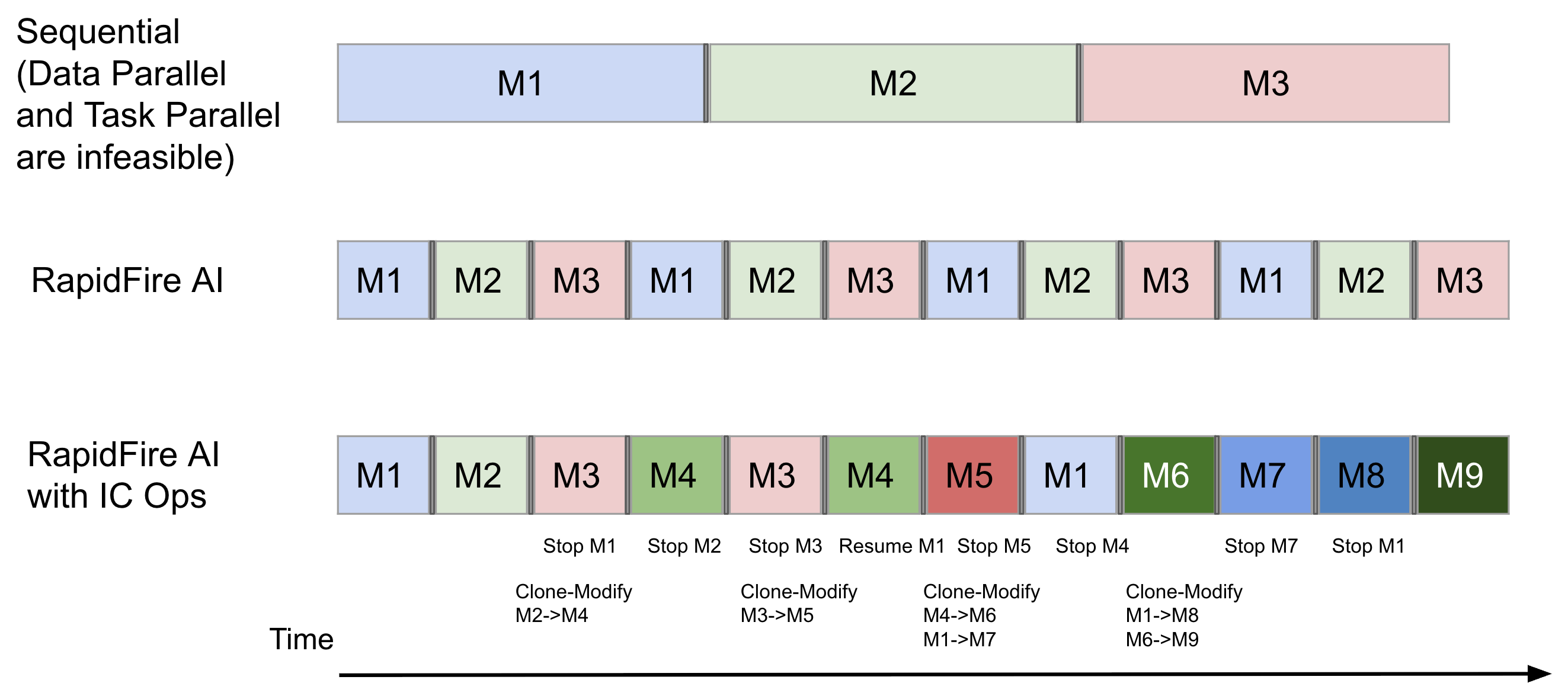 Sequential vs. RapidFire AI on a single GPU with chunk-based scheduling and IC Ops.
Installation and Setup
Option 1: Run in Google Colab
💡 Try RapidFire AI instantly in your browser with our adapted Google Colab notebook version of this tutorial. It is configured to run end-to-end in Colab with no local installation required.

Option 2: Run Locally
First, install RapidFire AI and authenticate with Hugging Face:
# Install RapidFire AI
!pip install rapidfireai

# Authenticate with Hugging Face
from huggingface_hub import login
login(token="YOUR_HF_TOKEN")  # Or use huggingface-cli login
Initialize and start the RapidFire AI server:
# Initialize RapidFire AI (one-time setup)
rapidfireai init

# Start the server and dashboard
rapidfireai start
The dashboard will be available at http://localhost:3000 where you can monitor experiments in real-time.
 RapidFire AI establishes live three-way communication between your IDE, a metrics dashboard, and a multi-GPU execution backend
Load and Prepare the Dataset
We'll use the Bitext Customer Support dataset, which contains instruction-response pairs for training customer support chatbots. The full, runnable version of this code is also available in the RapidFire AI tutorial notebook (provided that you've installed RapidFire AI locally) rf-tutorial-sft-chatqa-lite.ipynb.
from datasets import load_dataset

# Load the customer support dataset
dataset = load_dataset("bitext/Bitext-customer-support-llm-chatbot-training-dataset")

# Select subsets for training and evaluation
train_dataset = dataset["train"].select(range(128))
eval_dataset = dataset["train"].select(range(100, 124))

# Shuffle for randomness
train_dataset = train_dataset.shuffle(seed=42)
eval_dataset = eval_dataset.shuffle(seed=42)

print(f"Training samples: {len(train_dataset)}")
print(f"Evaluation samples: {len(eval_dataset)}")
Training samples: 128
Evaluation samples: 24
Define the Data Formatting Function
RapidFire AI uses the standard chat format with prompt and completion fields. Here's how to format the customer support data:
def sample_formatting_function(row):
    """Format each example into chat format for SFT training."""
    SYSTEM_PROMPT = "You are a helpful and friendly customer support assistant. Please answer the user's query to the best of your ability."

    return {
        "prompt": [
            {"role": "system", "content": SYSTEM_PROMPT},
            {"role": "user", "content": row["instruction"]},
        ],
        "completion": [
            {"role": "assistant", "content": row["response"]}
        ]
    }
This creates a structured conversation format that the model will learn to follow during training.
Initialize the RapidFire AI Experiment
Every RapidFire AI experiment needs a unique name and mode:
from rapidfireai import Experiment

# Create experiment for fine-tuning
experiment = Experiment(
    experiment_name="exp1-chatqa-lite",
    mode="fit"  # Use "fit" mode for training, "evals" for evaluation
)
✅ Experiment 'exp1-chatqa-lite' initialized
📊 MLflow tracking enabled at http://localhost:3000
Define Custom Evaluation Metrics
Optionally define custom metrics to evaluate generated responses:
def sample_compute_metrics(eval_preds):
    """Compute ROUGE and BLEU scores for generated responses."""
    predictions, labels = eval_preds

    import evaluate
    rouge = evaluate.load("rouge")
    bleu = evaluate.load("bleu")

    rouge_output = rouge.compute(predictions=predictions, references=labels, use_stemmer=True)
    bleu_output = bleu.compute(predictions=predictions, references=labels)

    return {
        "rougeL": round(rouge_output["rougeL"], 4),
        "bleu": round(bleu_output["bleu"], 4),
    }
Define Multiple Configurations
This is where RapidFire AI shines. We'll define 4 different configurations to compare:
- 2 LoRA configurations (small adapter vs. large adapter)
- 2 learning rates (1e-3 vs. 1e-4)
Quick LoRA Primer
LoRA (Low-Rank Adaptation) is a parameter-efficient fine-tuning technique that adds small trainable matrices to frozen model layers instead of updating all weights. Key parameters:
r(rank): Dimensionality of the adapter matrices—higher values = more capacity but more memorylora_alpha: Scaling factor for LoRA weights (typically 2× the rank)target_modules: Which model layers to adapt (e.g., attention projections likeq_proj,v_proj)lora_dropout: Dropout rate for regularization
Define LoRA Configurations
from rapidfireai.fit.automl import List, RFGridSearch, RFModelConfig, RFLoraConfig, RFSFTConfig

# Two LoRA configs with different adapter capacities
peft_configs_lite = List([
    RFLoraConfig(
        r=8,                                    # Small adapter: rank 8
        lora_alpha=16,
        lora_dropout=0.1,
        target_modules=["q_proj", "v_proj"],    # Attention only
        bias="none"
    ),
    RFLoraConfig(
        r=32,                                   # Large adapter: rank 32
        lora_alpha=64,
        lora_dropout=0.1,
        target_modules=["q_proj", "k_proj", "v_proj", "o_proj"],  # Full attention
        bias="none"
    )
])
Define Model and Training Configurations
# 2 base models x 2 peft configs = 4 combinations in total
config_set_lite = List([
    RFModelConfig(
        model_name="TinyLlama/TinyLlama-1.1B-Chat-v1.0",  # 1.1B model
        peft_config=peft_configs_lite,
        training_args=RFSFTConfig(
            learning_rate=1e-3,  # Higher LR for very small model
            lr_scheduler_type="linear",
            per_device_train_batch_size=4,
            per_device_eval_batch_size=4,
            max_steps=128,
            gradient_accumulation_steps=1,   # No accumulation needed
            logging_steps=2,
            eval_strategy="steps",
            eval_steps=4,
            fp16=True,
        ),
        model_type="causal_lm",
        model_kwargs={"device_map": "auto", "torch_dtype": "auto", "use_cache": False},
        formatting_func=sample_formatting_function,
        compute_metrics=sample_compute_metrics,
        generation_config={
            "max_new_tokens": 256,
            "temperature": 0.8,  # Higher temp for tiny model
            "top_p": 0.9,
            "top_k": 30,         # Reduced top_k
            "repetition_penalty": 1.05,
        }
    ),
    RFModelConfig(
        model_name="TinyLlama/TinyLlama-1.1B-Chat-v1.0",  # 1.1B model
        peft_config=peft_configs_lite,
        training_args=RFSFTConfig(
            learning_rate=1e-4,  # Lower LR
            lr_scheduler_type="linear",
            per_device_train_batch_size=4,
            per_device_eval_batch_size=4,
            max_steps=128,
            gradient_accumulation_steps=1,   # No accumulation needed
            logging_steps=2,
            eval_strategy="steps",
            eval_steps=4,
            fp16=True,
        ),
        model_type="causal_lm",
        model_kwargs={"device_map": "auto", "torch_dtype": "auto", "use_cache": False},
        formatting_func=sample_formatting_function,
        compute_metrics=sample_compute_metrics,
        generation_config={
            "max_new_tokens": 256,
            "temperature": 0.8,  # Higher temp for tiny model
            "top_p": 0.9,
            "top_k": 30,         # Reduced top_k
            "repetition_penalty": 1.05,
        }
    )
])
How Config Expansion Works: When you pass a List() of LoRA configs to peft_config, RapidFire AI automatically creates one run for each combination. With 2 LoRA configs × 2 model configs (different learning rates), this produces 4 concurrent runs.
Define the Model Creation Function
This function loads the model and tokenizer for each configuration. It handles different model types (causal_lm, seq2seq_lm, masked_lm) based on the model_type knob in your config:
from transformers import AutoModelForCausalLM, AutoTokenizer, AutoModelForSeq2SeqLM, AutoModelForMaskedLM

def sample_create_model(model_config):
    """Function to create model object for any given config; must return tuple of (model, tokenizer)"""
    model_name = model_config["model_name"]
    model_type = model_config["model_type"]
    model_kwargs = model_config["model_kwargs"]

    if model_type == "causal_lm":
        model = AutoModelForCausalLM.from_pretrained(model_name, **model_kwargs)
    elif model_type == "seq2seq_lm":
        model = AutoModelForSeq2SeqLM.from_pretrained(model_name, **model_kwargs)
    elif model_type == "masked_lm":
        model = AutoModelForMaskedLM.from_pretrained(model_name, **model_kwargs)
    elif model_type == "custom":
        # Handle custom model loading logic, e.g., loading your own checkpoints
        # model = ...
        pass
    else:
        # Default to causal LM
        model = AutoModelForCausalLM.from_pretrained(model_name, **model_kwargs)

    tokenizer = AutoTokenizer.from_pretrained(model_name)

    return (model, tokenizer)
Create the Config Group
RapidFire AI uses RFGridSearch to generate a Config Group—a set of configurations produced from all combinations of your knobs. Each configuration in the Config Group later becomes a separate run on the GPU:
# Create a config group using grid search
config_group = RFGridSearch(
    configs=config_set_lite,
    trainer_type="SFT"  # Use SFT trainer
)
Run Concurrent Training
Now execute the training with chunk-based scheduling:
# Launch concurrent training of all 4 runs
experiment.run_fit(
    config_group,
    sample_create_model,
    train_dataset,
    eval_dataset,
    num_chunks=4,  # Split data into 4 chunks for interleaved execution
    seed=42
)
What is
num_chunks? RapidFire AI splits your dataset into chunks and trains all runs on each chunk before moving to the next; this training pattern is called chunk-based scheduling. This enables early comparison—after chunk 1 completes, you can already see which runs are performing better, instead of waiting for full training. Use 4-8 chunks for most experiments.
🚀 Starting RapidFire AI training...
📊 4 configurations detected → 4 runs created
📦 Dataset split into 4 chunks

[Chunk 1/4] Training all runs on samples 0-32...
  Run 1 (r=8, lr=1e-3):  loss=2.45
  Run 2 (r=32, lr=1e-3): loss=2.38
  Run 3 (r=8, lr=1e-4):  loss=2.52
  Run 4 (r=32, lr=1e-4): loss=2.49

[Chunk 2/4] Training all runs on samples 32-64...
  Run 1: loss=1.89 ↓
  Run 2: loss=1.72 ↓  ← Leading!
  Run 3: loss=2.31 ↓
  Run 4: loss=2.18 ↓

...

✅ Training complete in 12 minutes
📊 Results available at http://localhost:3000
What Happens During Execution
- Config Expansion: 4 configurations expand into 4 runs (one run per configuration)
- Chunk-based Scheduling: Data is split into chunks; all runs train on each chunk before moving to the next
- GPU Swapping: Models efficiently swap in/out of GPU memory at chunk boundaries
- Real-time Metrics: View all training curves simultaneously in the dashboard
- IC Ops Available: Stop, Resume, Clone-Modify, or Delete any run mid-training
End the Experiment
Always close the experiment to finalize logging:
experiment.end()
✅ Experiment 'exp1-chatqa-lite' completed
📁 Checkpoints saved to ./exp1-chatqa-lite/
📊 Full results available in MLflow dashboard
Analyzing Results
After training, you can compare all runs in the MLflow dashboard. Example results:
| Run | LoRA Rank | Learning Rate | Final Loss | ROUGE-L | BLEU |
|---|---|---|---|---|---|
| 1 | 8 | 1e-3 | 1.42 | 0.65 | 0.28 |
| 2 | 32 | 1e-3 | 1.21 | 0.72 | 0.34 |
| 3 | 8 | 1e-4 | 1.89 | 0.58 | 0.22 |
| 4 | 32 | 1e-4 | 1.67 | 0.63 | 0.27 |
Insight: Run 2 (larger LoRA rank + higher learning rate) converges fastest and achieves the best metrics for this task.
Interactive Control Operations (IC Ops)
During training, you can use IC Ops from the dashboard to dynamically control runs in flight. RapidFire AI supports 4 IC Ops:
- Stop: Terminate underperforming runs early to save compute
- Resume: Restart a previously stopped run
- Clone-Modify: Duplicate a promising run with modified hyperparameters (optionally warm-start from the parent's weights)
- Delete: Remove a run entirely from the experiment
 Clone-Modify a promising run with modified hyperparameters, optionally warm-starting from the parent's weights, all from the live dashboard
This enables adaptive experimentation where you react to results in real-time instead of waiting for all training to complete.
Benchmarks: Time Savings
Here's what you can expect when switching from sequential to RapidFire AI concurrent training:
| Scenario | Sequential Time | RapidFire AI | Speedup |
|---|---|---|---|
| 4 configs, 1 GPU | 120 min | 7.5 min | 16× |
| 8 configs, 1 GPU | 240 min | 12 min | 20× |
| 4 configs, 2 GPUs | 60 min | 4 min | 15× |
Benchmarks on NVIDIA A100 40GB with TinyLlama-1.1B and Llama-3.2-1B models
🎉 Conclusion
This tutorial demonstrated how RapidFire AI transforms SFT experimentation from a slow, sequential process into fast, parallel exploration:
- Define a Config Group: Use
List()wrappers to specify multiple configurations - Run Concurrently:
RFGridSearchorchestrates all runs with chunk-based scheduling - Monitor Live: Real-time dashboard shows all training curves simultaneously
- Adapt Mid-Flight: IC Ops let you stop underperforming runs and clone-modify promising ones
The Result: You can compare 4-8 runs in the time it previously took to train just one, enabling you to find better models faster and more efficiently.
🚀 Next Steps
- Try Different Models: Replace TinyLlama with Llama-3.2-1B, Qwen2-0.5B, or Phi-3-mini
- Expand the Grid: Add more learning rates, LoRA ranks, or target modules
- Use Full Dataset: Scale up from 128 to 10K+ samples for production training
- Explore DPO/GRPO: Use
RFDPOConfigorRFGRPOConfigfor preference alignment
📚 Resources
- 🚀 Try it hands-on: Interactive Colab Notebook
- 📖 Documentation: oss-docs.rapidfire.ai
- 💻 GitHub: RapidFireAI/rapidfireai
- 📓 Full SFT Tutorial: rf-tutorial-sft-chatqa-lite.ipynb
- 📖 TRL Integration: Hugging Face TRL RapidFire Integration
- 💬 Community: Discord — Get help and share results